Paper Review: No Free Lunch Theorem, Inductive Skepticism, and the Optimality of Meta-induction

The infamous no free lunch theorem (NFL theorem) asserts that all computable prediction methods have equal expected success. Computer scientists, and occasionally philosophers, often describe this result as a computer-science cousin of Hume’s problem of induction.

Given this theorem, one might think that trying to design a better or worse prediction algorithm for general prediction tasks is pointless: you might as well just design one that guesses randomly, for you will expect it to do just as well as any sophisticated method you could devise.

However, things aren’t so simple. There is also a result from the literature on meta-induction that, in the long run, certain kinds of meta-inductors–predictors that can use the predictions of other predictions to help make their own predictions–can dominate other methods.

So, it seems like it is both the case that no predictor can do better than another in general, and yet that there are some predictors that do better (or at least as good as) others, in general. What is going on here?

This is the central question of Gerhard Schurz’s paper No Free Lunch Theorem, Inductive Skepticism, and the Optimality of Meta-induction.

***The original paper can be found here.***

As you might have expected, Schurz shows that there is in fact no contradiction between these results. As usual, once we more clearly understand the details of the results, the tension vanishes. However, I think that the specific way in which the tension vanishes in this case gets at some deep concepts and issues in formal epistemology.

First, let’s get a better understand of what exactly the NFL theorem says. Schurz notes that there are really two forms of the theorem: the strong form and the weak form. I’ll first outline the general context in which the theorems apply, then I’ll consider both versions.

The context is that of a prediction game: we have a sequence of outcomes, for example, , and the goal is to predict this sequence well. That is, after the first terms of the sequence, we want to predict the term.

We might wonder what kind of outcomes and predictions are allowed. For example, in the above sequence, the only outcomes we saw were s and s . In general, for Schurz the possible outcomes in each prediction game will be a subset Val of the interval , However, for ease of thinking about it, I will mainly talk about the case where Val . The possible values that we can predict will be a superset of Val. For example, we might be able to predict just 0 or 1, or we might be allowed to predict any real number in the interval (this is useful if we want to think of the prediction game as guessing the probability that the next digit is a 0 or a 1).

When a prediction is made of the next outcome in a sequence, we evaluate how well the predictor did by scoring its prediction using a loss function. For example, we might score the predictor by the difference between its prediction and the true value. In this case if the predictor predicted 0.7, and the digit was a 1, then it receives a loss of 0.3.

For the NFL theorem we restrict the kind of predictors we will allow for computable ones. Each predictor will be a function from the past n outcomes to a future n+1th prediction.

Consider all of the possible sequences of observations we could have. In the binary case where the only observations are 0 and 1, this corresponds to the set of all infinite binary strings. One of the assumptions needed for both the strong and the weak versions of the NFL theorem is a state-uniform prior probability over all possible outcome sequences.

What exactly does this mean? It means that for all natural numbers n, the probability of each sequence of length n is equal. For example, if n=2, then each of the four sequences

00
01
10
11

is equally likely. Once we have this for finite n, it can be extended to the infinite case using a little more sophisticated mathematics. The main thing to keep in mind here is that the prior probability over sequences of outcomes is uniform.

As I briefly mentioned earlier, we use a loss function to evaluate difference predictors. The difference between the weak and the strong NFL theorems turn on the types of loss functions we allow.

For the strong NFL theorem, we allow only homogeneous loss functions. A loss function is homogeneous if, for each possible loss value c, the number of possible outcome (for example, 0 or 1) that lead to a loss of c for a certain prediction pred is the same for each possible prediction.

This seems a little opaque, but consider the case where the possible events are 0 and 1, the only possible predictions are 0 and 1, and we give a predictor a loss of 0 if its prediction is correct and 1 if it is incorrect. Then this loss function is homogeneous, because for both predictions 0 and 1, the number of possible events that lead to a loss of 1 is 1, and the number that lead to a loss of 0 is one. For if the outcome we wanted to predict was 0, then predicting 0 would have a loss of 0 and predicting 1 would have a loss of 1. If the outcome we wanted to predict was 1, then predicting 1 would have a loss of 0 and predicting 0 would have a loss of 1. We can see then how this is a homogeneous loss function. Though most loss functions are not homogeneous, if the one we are using is homogeneous the following holds:

For every possible loss value c, the probability of worlds in which the prediction method leads to a loss of c is the same for all possible prediction methods. (Schurz, p. 830) F

Informally, this theorem says that for a pair of prediction methods, the probability of getting a sequence in which the first outperforms the second is the same as the probability in which the second outperforms the first.

The weak theorem places less of a constraint on the type of loss functions allowed, requiring them to only be weakly homogeneous. The exact details of a weakly homogeneous loss function can be found in the paper (it’s not terribly complicated, but inessential for our story here). If one allows only weakly homogeneous loss functions we get the following result:

The probabilistically expected success of every possible prediction method is equal to the expected success of random guessing or of every other prediction method. (Schurz, p. 831)

Informally, this says that any possible computable prediction method has the same expected predictive success (given a uniform prior over the possible sequences of observations). Schurz restricts his analysis to cases in which the weak NFL theorem applies. He writes

For all induction-friendly philosophical programs, including the program of meta-induction, this result seems to be devastating. How is it possible?  (p. 832)

In order to see how this seems to conflict with Schurz’s own results in meta-induction, let us turn to the meta-induction framework.

The idea of meta-induction is that we have a set of predictors which each output predictions, and a meta-inductor that is allowed to look at the predictions each of the other predictor makes, and then make its predictors using theirs. For example, a simple type of meta-inductor would be one that looks at the track record of each of the other predictors, observes what they predict, and then makes the same prediction as the predictor with the lowest overall loss so far.

We can think of the other predictors as friends that the meta-inductor has that it asks, experts in a field whose work it reads, or even different physical theories or statistical models that it considers. It then aggregates the different predictions of each of these in order to come up with a good prediction of its own.

Schurz showed in an earlier paper that the provably universally optimal meta-inductive strategy is attractivity-weighted meta-induction (wMI). The attractivity of a different predictor is the difference between how successful the predictor has been and how successful the meta-inductor has been. The prediction of wMI is then a weighted average of the other predictors’ predictions in which the weights are the attractivity of the other predictors. The mathematical details are in the paper for those of you who are curious. The important thing to take away here is that wMI keeps track of how successful the other predictors are, and then combines their predictions into one meta-prediction that is optimal.

What exactly does optimal mean here? We have the answer in the following theorem, which holds for every prediction game and every finite set of predictors in which wMI is the only meta-inductor:

(1) Short run: for all  
(2) Long run: (strictly) converges to the non-MI-predictors’ maximal success for .

where is the success of a predictor, and m is the number of non-MI predictors.

The short run result says that the difference between the best non-MI predictor success and the success of wMI’s does not differ too much. The long run result says that in the limit, as we consider more and more of the sequence, wMI will do at least as well as the best other predictor. More of the technical details are in the paper.

Thus, it seems like we have a puzzle: on the one hand the NFL theorem says that each predictor performs equally well (in expectation), while on the other we have that wMI is universally optimal. What are we to make of this?

Schurz has the answer: it is the assumption of a uniform prior that is driving the result.

The details are a little bit technical, but here is the thrust of the observation. When we take a uniform prior over possible sequences, we can think of this as taking a uniform prior probability density over the unit interval, since each real number between 0 and 1 can be written as an infinite binary string. This might seem like a natural prior—each sequence is equal likely. However, Schurz notices that this is hiding something. The assumption of such a uniform prior over sequences leads to a prior probability of 1 on the limiting relative frequency of the sequence being . Informally, this is the assumption that the seqeunce is made up of an equal number of 0s and 1s. We see this relationship in the following helpful figure from Schurz.

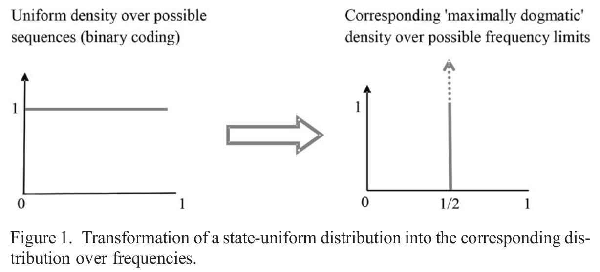
This is a very strong assumption. Far from reflecting a lack of knowledge in how the world will be, this is assuming that the sequence has a very specific limiting relative frequency, and contains no patterns whatsoever. You can think of this as a sequence generated by flipping a fair coin infinitely often, and recording a 0 when you see tails and a 1 when you see heads.

Thus, Schurz points out, this gives us the insight into why the two theorems do not conflict. The NFL theorem assumes that there is no pattern in the sequence—of course no prediction method will do better than any other on average! There is no pattern it could pick up!

We can see this by considering an example. Suppose the sequence so far has been

11111111111111111

We might think it likely that the next digit will be a 1. However, since NFL assumes that each sequence of the same length is as likely as any other, we see that

111111111111111110

is as likely as

111111111111111111

under the assumptions of the theorem. This means that the predictor noticing the pattern of all 1s has no advantage over one that guesses randomly. And it is true. But it is true because of the assumed distribution. This is what is doing the work. It makes learning impossible. If we take different prior probabilities over possible sequences we do not get the same result.

What this assumption does is rule out sequences with patterns. These are precisely the ones in which wMI can do well, for it tracks the success of other prediction methods. There is no contradiction between the theorems; it is simply by assuming the uniform prior over sequences that the NFL theorem rules out the sequences on which wMI excels.

Furthermore, it seems that the meta-inductive framework is capturing more of what we want. We want to use methods, such that, if there is a pattern, they will detect it. The meta-induction result is a step in the right direction. Though the NFL theorem is true, once we understand the assumptions that go into it, it is underwhelming.